29. Bayesian ANOVA
Parameter estimation & hypothesis testing
2025-11-14
What is a model?
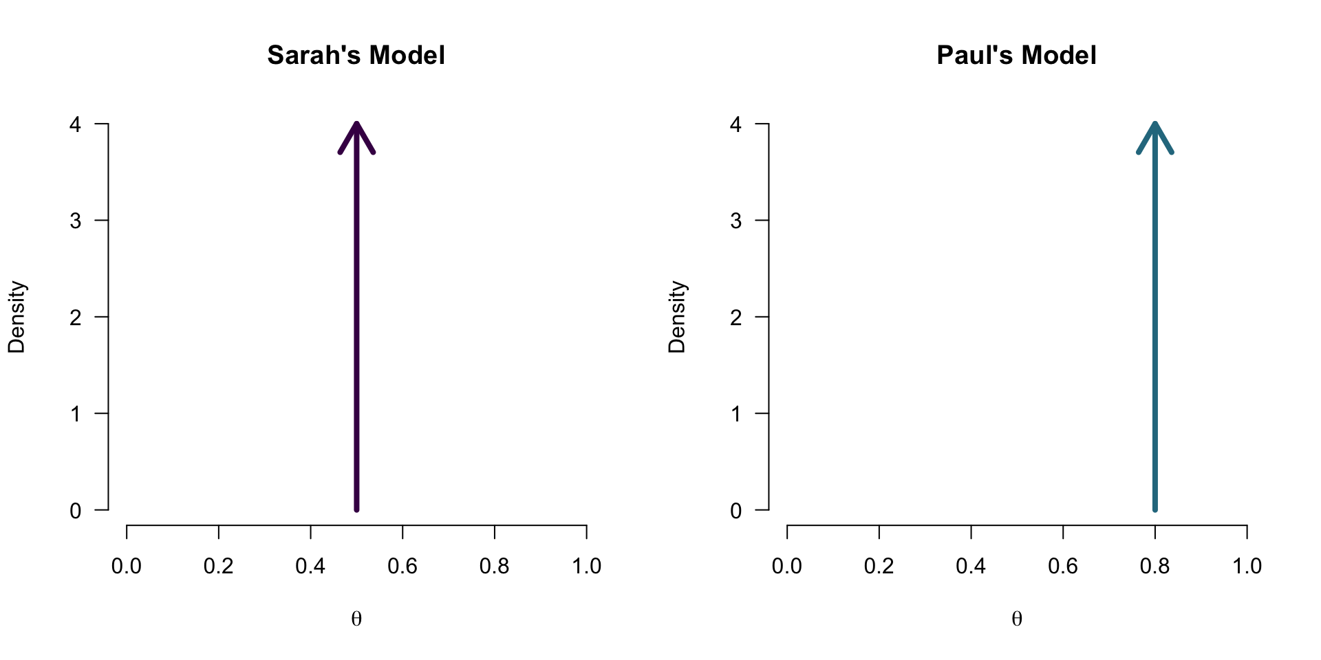
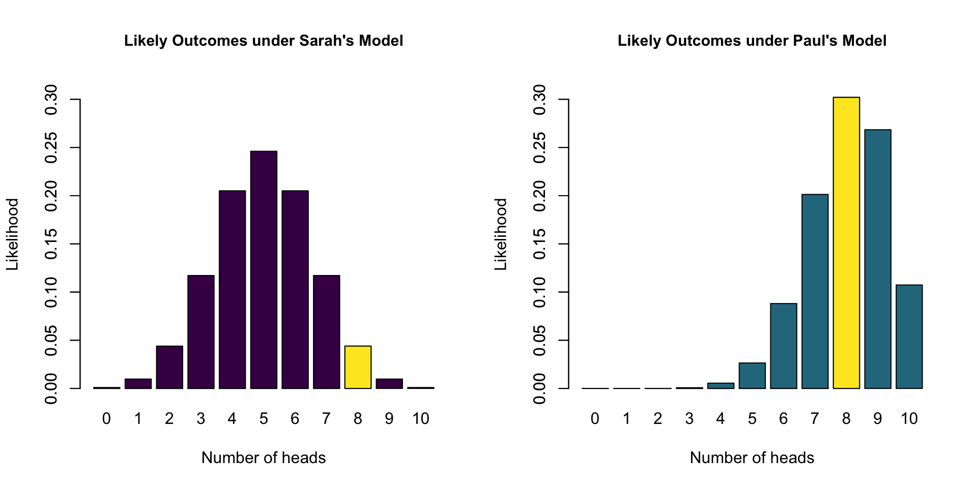
What does a model predict?
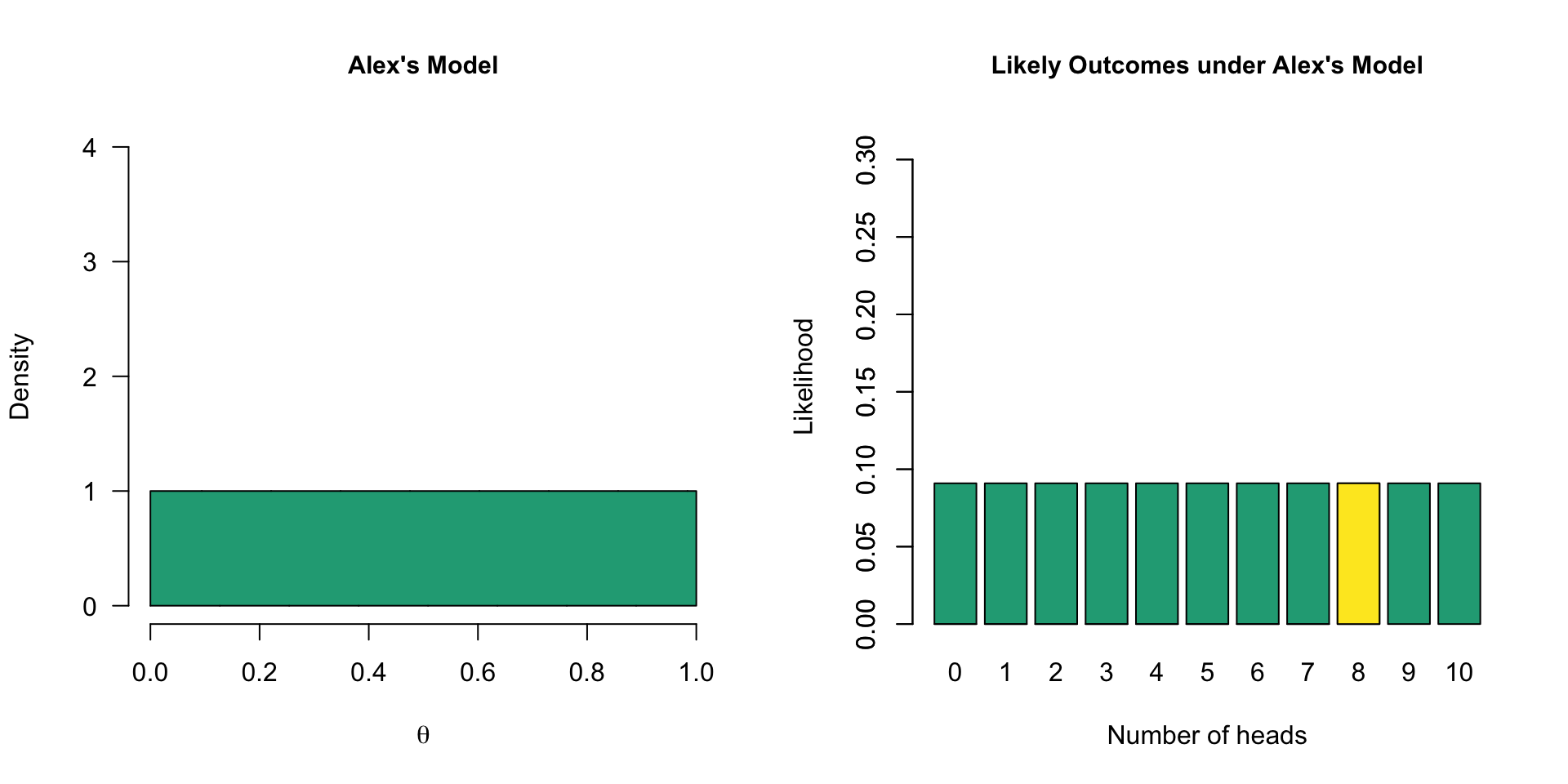
Model with multiple values
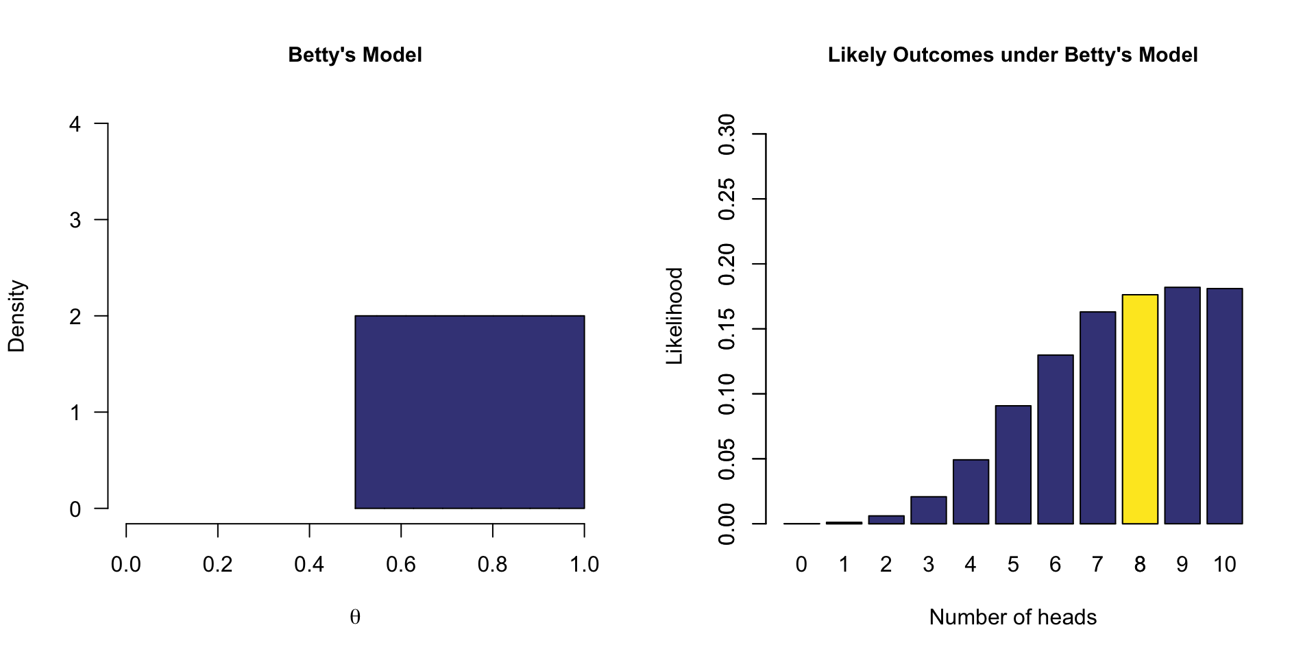
One-sided model
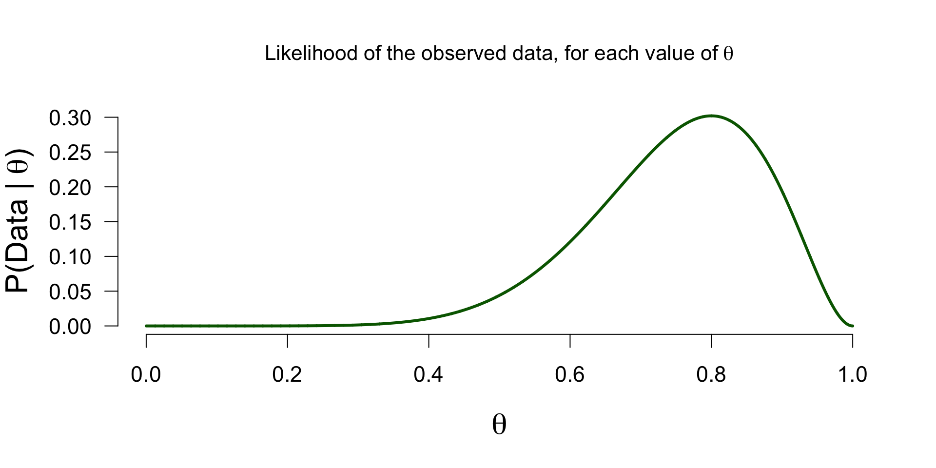
Likelihood function - \(P(data | \theta)\)
How likely is 8 out of 10 for all possible \(\theta\) values?
\[\binom{n}{k} \theta^k (1-\theta)^{n-k}\]
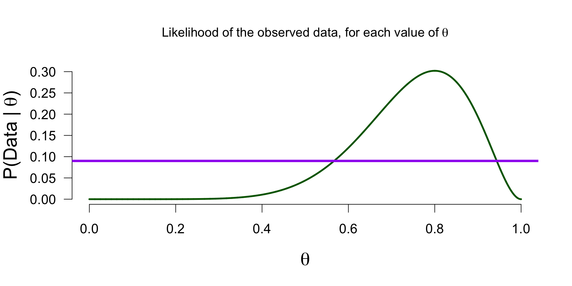
Marginal likelihood - \(P(data)\)
How likely is 8 out of 10 for all \(\theta\) values in the model, on average?
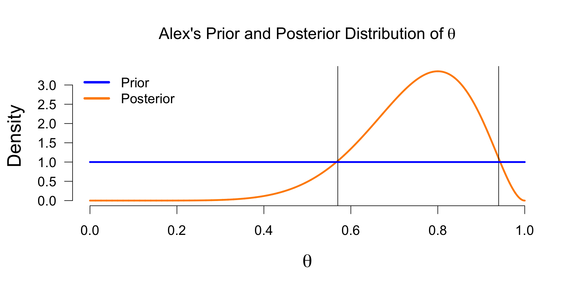
Updating beliefs
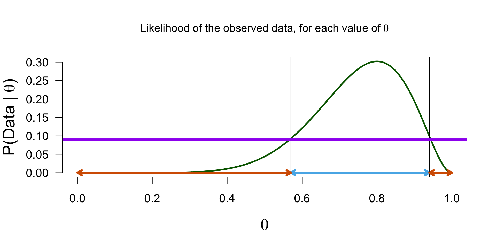
Posterior distribution - \(P(\theta | data)\)
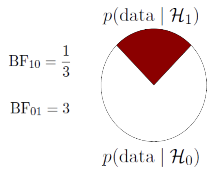
Bayes Factor
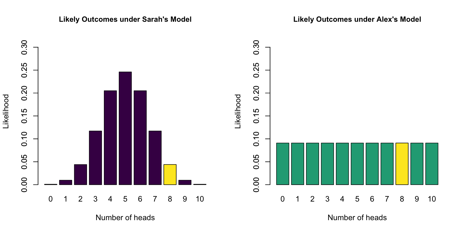
- Sarah’s model has a marginal likelihood of 0.04 for 8 heads
- Alex’s model has a marginal likelihood of 0.09 for 8 heads
- \(\text{BF}_{SA} =\) 0.04 / 0.09 = 0.44
- The data are 0.44 times more likely under Sarah’s model than under Alex’s model
- The data are 2.25 times more likely under Alex’s model than under Sarah’s model
BF pizza
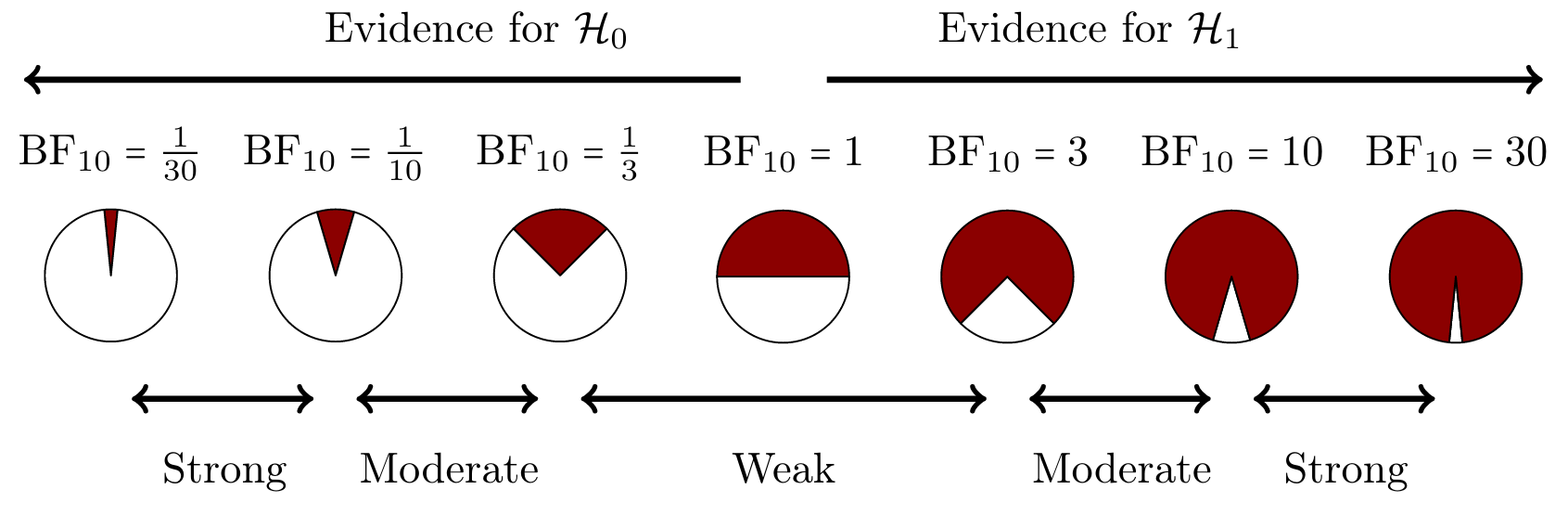
BF pizza
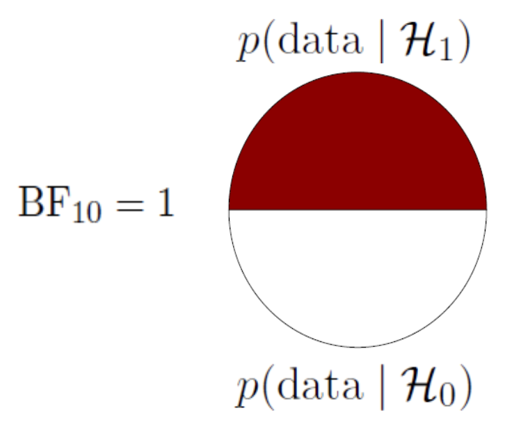
BF pizza
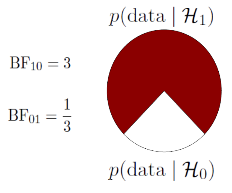
BF pizza
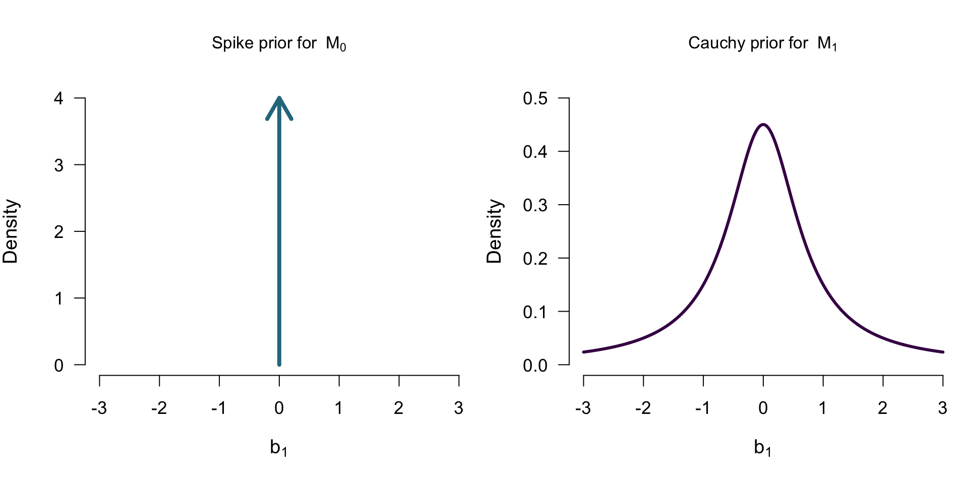
Two Models
\[\mathcal{M_0}: b_1 = 0 \] \[\mathcal{M_1}: b_1 \sim Cauchy(0.707)\]
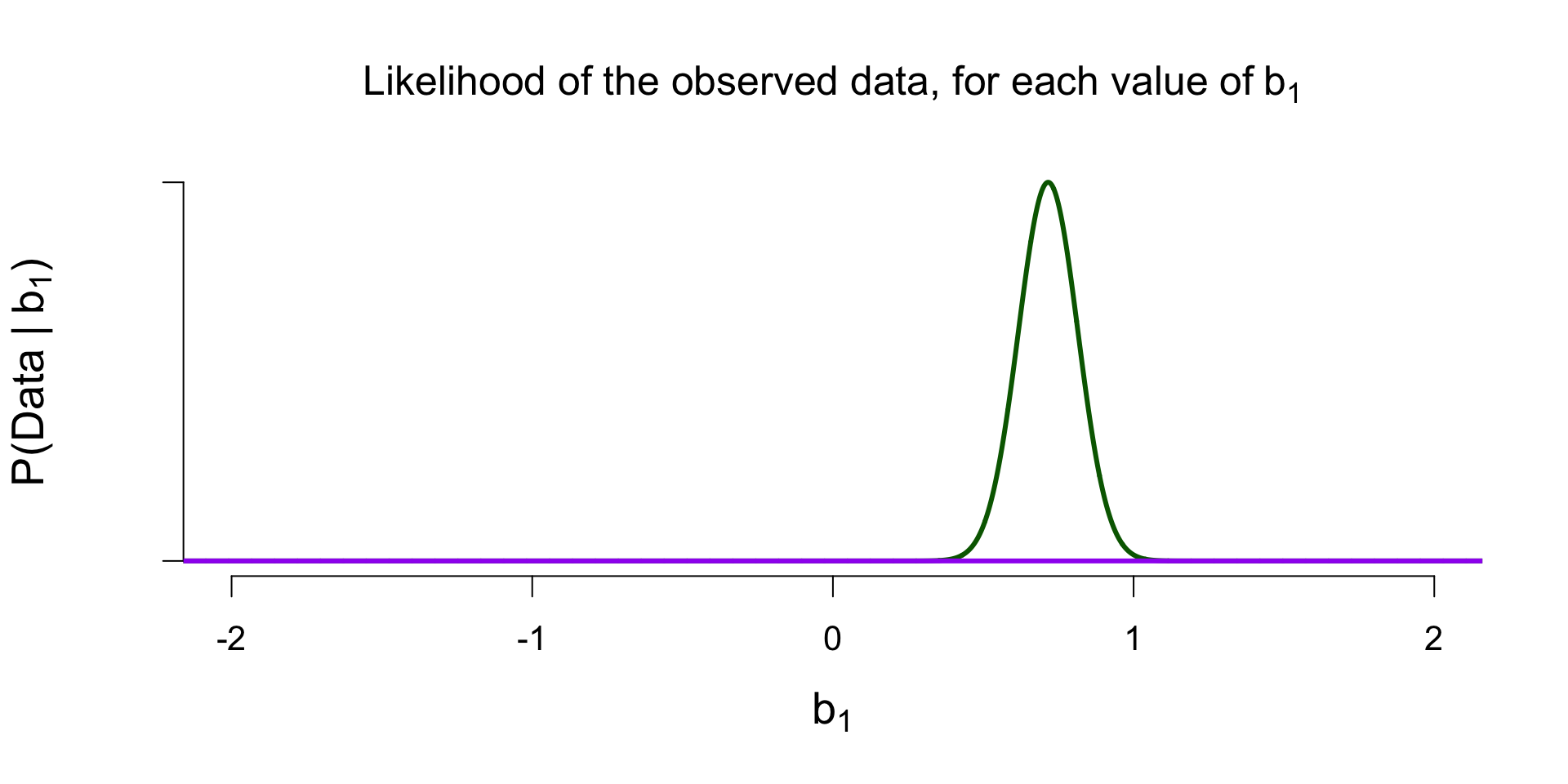
Marginal Likelihood of \(\mathcal{M}_1\)
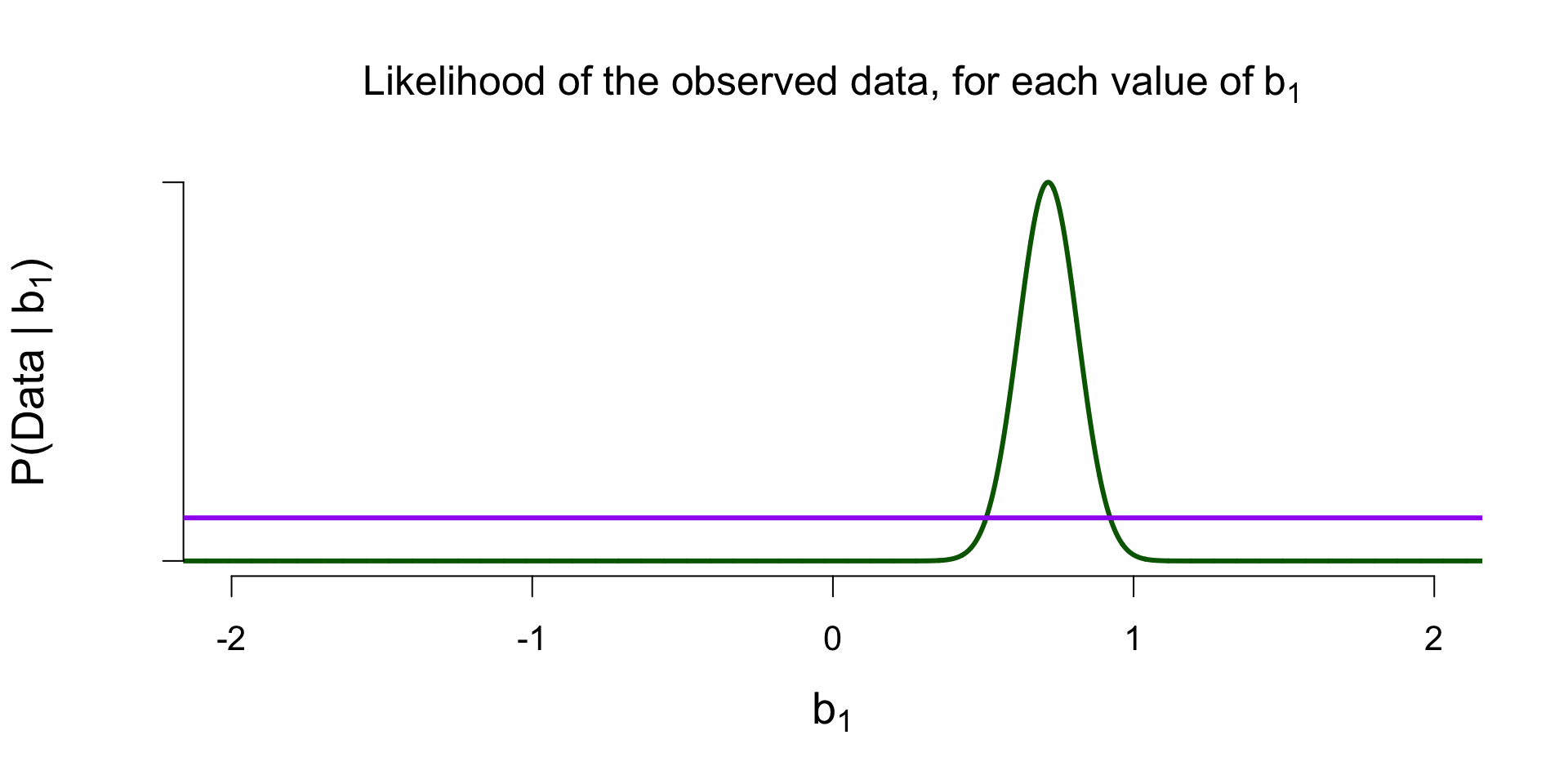
Marginal Likelihood of \(\mathcal{M}_0\)
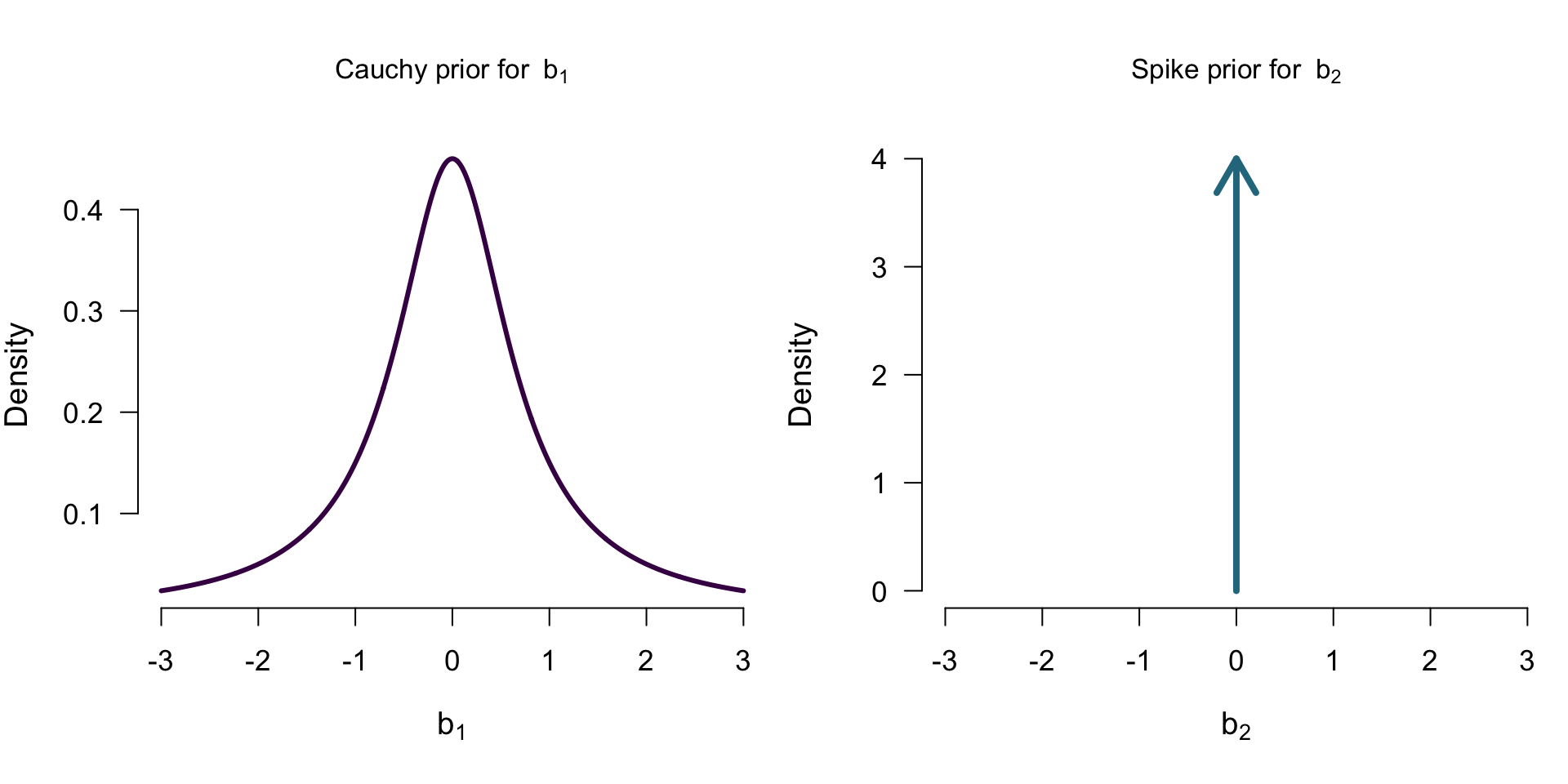
Priors for \(\mathcal{M_A}\)
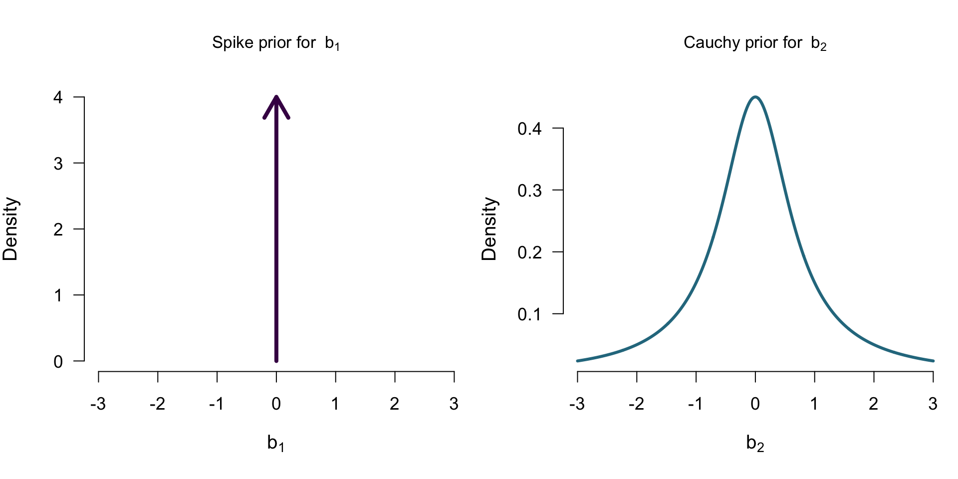
Priors for \(\mathcal{M_C}\)
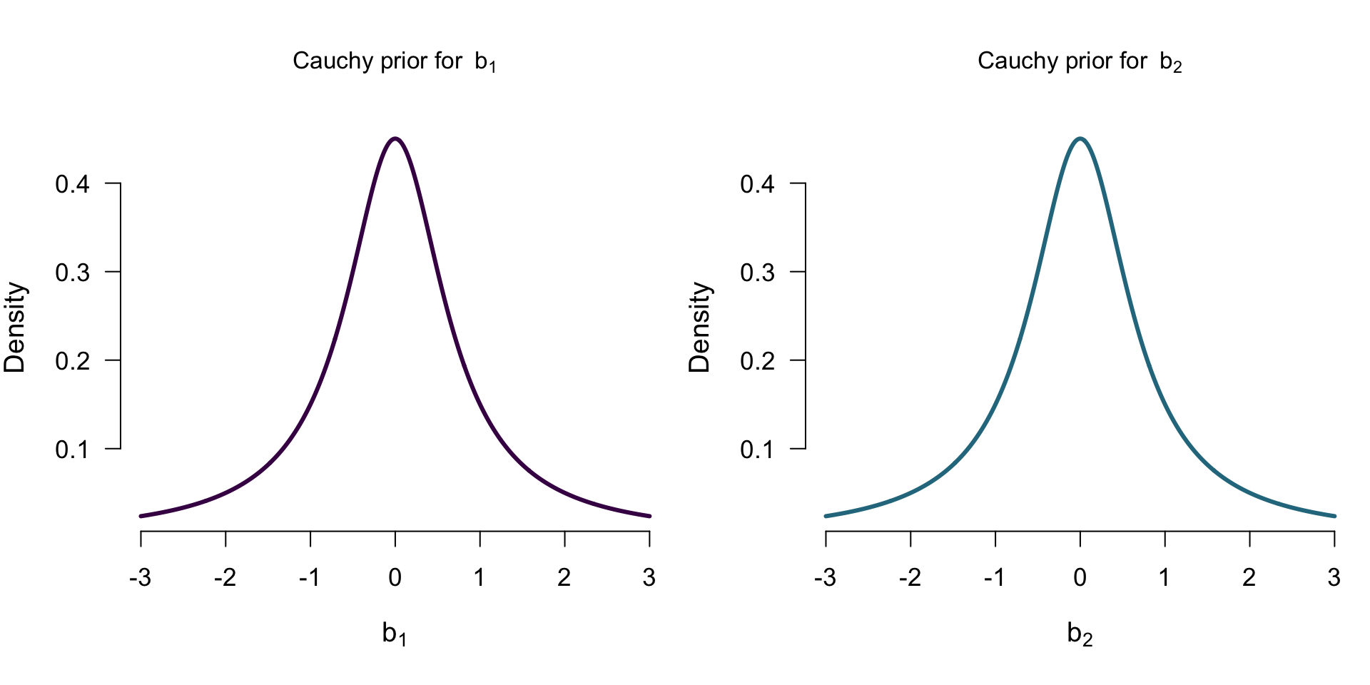
Priors for \(\mathcal{M_{A+C}}\)
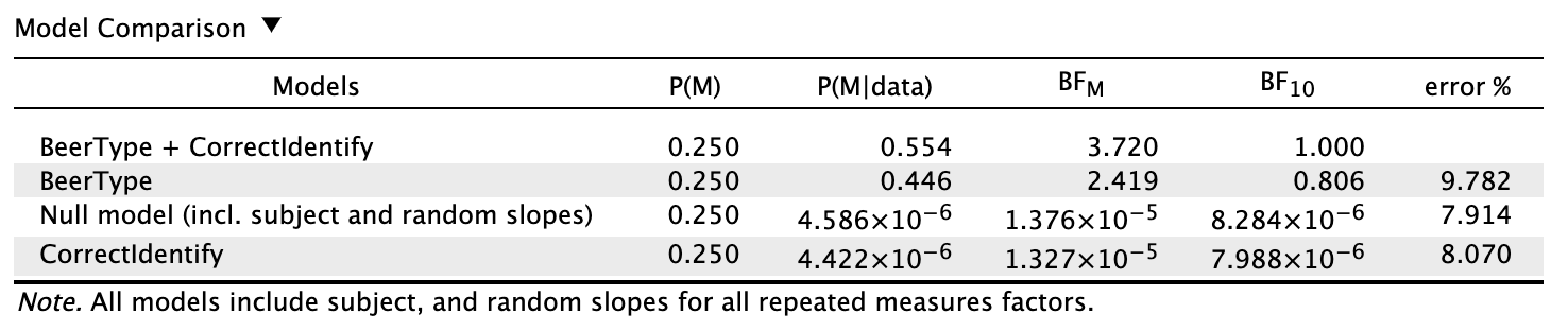
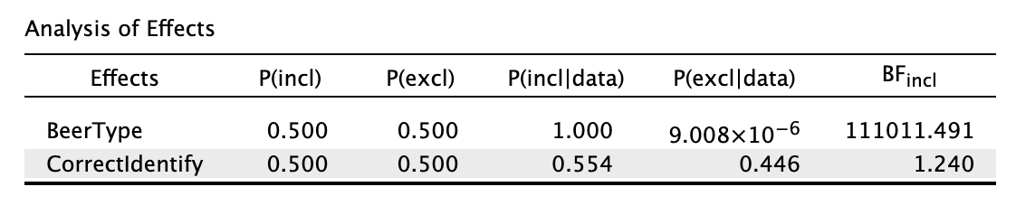
Model comparison results
Looking at the individual effects
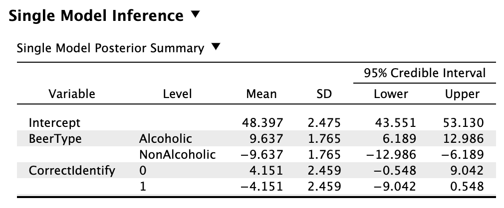
Single model inference
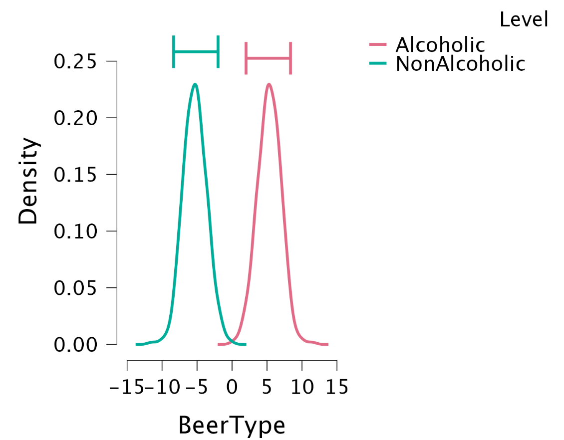
Single model inference: Posterior for BeerType
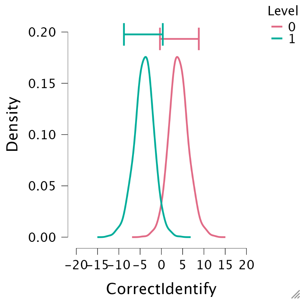
Single model inference: Posteriors for CorrectIdentify
Lost?

JASP
![]()
Contact

![]()